Run inference on time series of Sentinel-2 images
Contents
Run inference on time series of Sentinel-2 images#
Last Modified: 15-03-2022
Author: Gonzalo Mateo-García
This notebook shows how to query time series of images of Sentinel-2 over an area of interest (AoI) between two dates using the Google Earth Engine. Hence to run this notebook you a Google Earth Engine account.
We show how to export those images to the Google Drive or to a Google bucket and we run inference on them to produce flood segmentation maps that are vectorized and shown in an interactive map.
Note: If you run this notebook in Google Colab change the running environment to use a GPU.
from datetime import datetime, timedelta, timezone
import geopandas as gpd
import pandas as pd
import ee
import geemap.eefolium as geemap
import folium
from ml4floods.data import ee_download
from shapely.geometry import mapping, shape
import matplotlib.pyplot as plt
import os
Step 1: Config AoI and dates to search for S2 images#
You can test this notebook on a different AoI and dates, just change those variables in the cell bellow for this.
date_event = datetime.strptime("2021-02-12","%Y-%m-%d").replace(tzinfo=timezone.utc)
date_start_search = datetime.strptime("2021-01-15","%Y-%m-%d").replace(tzinfo=timezone.utc)
date_end_search = date_start_search + timedelta(days=45)
area_of_interest_geojson = {'type': 'Polygon',
'coordinates': (((19.483318354000062, 41.84407200000004),
(19.351701478000052, 41.84053242300007),
(19.298659824000026, 41.871157520000054),
(19.236388306000038, 41.89588351100008),
(19.22956438700004, 42.086957306000045),
(19.327827977000027, 42.09102668200006),
(19.778082109000025, 42.10312055000003),
(19.777652446000047, 41.97309238100007),
(19.777572772000042, 41.94912981900006),
(19.582705341000064, 41.94398333100003),
(19.581417139000052, 41.94394820700006),
(19.54282145700006, 41.90168177700008),
(19.483318354000062, 41.84407200000004)),)}
area_of_interest = shape(area_of_interest_geojson)
def generate_polygon(bbox):
"""
Generates a list of coordinates: [[x1,y1],[x2,y2],[x3,y3],[x4,y4],[x1,y1]]
"""
return [[bbox[0],bbox[1]],
[bbox[2],bbox[1]],
[bbox[2],bbox[3]],
[bbox[0],bbox[3]],
[bbox[0],bbox[1]]]
Step 2: Plot cloud coverage of available S2 image over AoI and search dates#
Next cell obtains the time series of S2 images over the provided AoI. This is a ee.ImageCollection object (img_col variable). Afterwards it obtains for each image the time of acquisition (system:time_start), the number of valid pixels (valids), and the average cloud probability (cloud_probability) in a pandas DataFrame (img_col_info_local). With this dataframe we plot the average cloud probability.
The cloud probability is obtained from the s2cloudless model which is available in the Google Earth Engine as an independent collection.
ee.Initialize()
bounds_pol = generate_polygon(area_of_interest.bounds)
pol_2_clip = ee.Geometry.Polygon(bounds_pol)
pol = ee.Geometry(area_of_interest_geojson)
# Grab the S2 images and the Permanent water image
img_col = ee_download.get_s2_collection(date_start_search,
date_end_search, pol)
permanent_water_img = ee_download.permanent_water_image(date_event.year, pol_2_clip)
# Get info of the S2 images (convert to table)
img_col_info = ee_download.img_collection_to_feature_collection(img_col,
["system:time_start", "valids", "cloud_probability"])
img_col_info_local = gpd.GeoDataFrame.from_features(img_col_info.getInfo())
img_col_info_local["valids"]*=100
img_col_info_local["system:time_start"] = img_col_info_local["system:time_start"].apply(lambda x: datetime.utcfromtimestamp(x/1000))
n_images_col = img_col_info_local.shape[0]
print(f"Found {n_images_col} S2 images between {date_event.isoformat()} and {date_end_search.isoformat()}")
plt.figure(figsize=(15,5))
plt.plot(img_col_info_local["system:time_start"], img_col_info_local["cloud_probability"],marker="x")
plt.ylim(0,101)
plt.xticks(rotation=30)
plt.ylabel("mean cloud coverage % over AoI")
plt.grid(axis="x")
Found 18 S2 images between 2021-02-12T00:00:00+00:00 and 2021-03-01T00:00:00+00:00
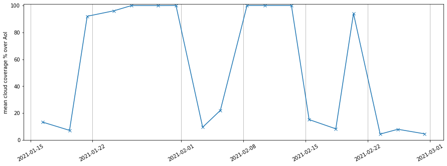
DataFrame with date of acquisition, averaged cloud probability and percentage of valid pixels.
img_col_info_local
| geometry | cloud_probability | system:time_start | valids | |
|---|---|---|---|---|
| 0 | POLYGON ((-180.00000 -90.00000, 180.00000 -90.... | 13.254181 | 2021-01-16 09:38:59.983 | 100 |
| 1 | POLYGON ((-180.00000 -90.00000, 180.00000 -90.... | 7.172355 | 2021-01-19 09:48:56.039 | 100 |
| 2 | POLYGON ((-180.00000 -90.00000, 180.00000 -90.... | 91.966141 | 2021-01-21 09:39:00.993 | 100 |
| 3 | POLYGON ((-180.00000 -90.00000, 180.00000 -90.... | 96.029202 | 2021-01-24 09:48:56.823 | 100 |
| 4 | POLYGON ((-180.00000 -90.00000, 180.00000 -90.... | 99.941818 | 2021-01-26 09:39:00.106 | 100 |
| 5 | POLYGON ((-180.00000 -90.00000, 180.00000 -90.... | 99.897624 | 2021-01-29 09:48:55.986 | 100 |
| 6 | POLYGON ((-180.00000 -90.00000, 180.00000 -90.... | 100.000000 | 2021-01-31 09:39:00.341 | 100 |
| 7 | POLYGON ((-180.00000 -90.00000, 180.00000 -90.... | 9.503629 | 2021-02-03 09:48:55.943 | 100 |
| 8 | POLYGON ((-180.00000 -90.00000, 180.00000 -90.... | 22.013119 | 2021-02-05 09:38:59.531 | 100 |
| 9 | POLYGON ((-180.00000 -90.00000, 180.00000 -90.... | 99.999951 | 2021-02-08 09:48:55.218 | 100 |
| 10 | POLYGON ((-180.00000 -90.00000, 180.00000 -90.... | 99.999130 | 2021-02-10 09:38:59.013 | 100 |
| 11 | POLYGON ((-180.00000 -90.00000, 180.00000 -90.... | 100.000000 | 2021-02-13 09:48:54.985 | 100 |
| 12 | POLYGON ((-180.00000 -90.00000, 180.00000 -90.... | 15.191459 | 2021-02-15 09:38:58.363 | 100 |
| 13 | POLYGON ((-180.00000 -90.00000, 180.00000 -90.... | 8.315460 | 2021-02-18 09:48:53.845 | 100 |
| 14 | POLYGON ((-180.00000 -90.00000, 180.00000 -90.... | 94.017820 | 2021-02-20 09:38:59.706 | 100 |
| 15 | POLYGON ((-180.00000 -90.00000, 180.00000 -90.... | 4.401171 | 2021-02-23 09:48:55.862 | 100 |
| 16 | POLYGON ((-180.00000 -90.00000, 180.00000 -90.... | 7.978288 | 2021-02-25 09:38:58.740 | 100 |
| 17 | POLYGON ((-180.00000 -90.00000, 180.00000 -90.... | 4.595103 | 2021-02-28 09:48:55.012 | 100 |
Step 3: Display S2 images over the AoI#
In the next cell we loop over the available S2 images and show those with low cloud coverage using the geemap package. If you see this notebook in the tutorial web page you will not seen the images; however if you run this cell with access to the GEE you’ll be able to see the Sentinel-2 images in the interactive map!
Map = geemap.Map()
imgs_list = img_col.toList(n_images_col, 0)
for i in range(n_images_col):
if img_col_info_local.iloc[i]["cloud_probability"] > 75:
continue
img_show = ee.Image(imgs_list.get(i))
Map.addLayer(img_show.clip(pol),
{"min":0, "max":3000,
"bands":["B11","B8","B4"]},
f"({i}/{n_images_col}) S2 SWIR/NIR/RED {img_col_info_local['system:time_start'][i].strftime('%Y-%m-%d')}",
True)
visualization = {
"bands": ['waterClass'],
"min": 0.0,
"max": 3.0,
"palette": ['cccccc', 'ffffff', '99d9ea', '0000ff']
}
Map.addLayer(permanent_water_img, visualization, name="JRC Permanent water")
Map.addLayer(pol, {"color": 'FF000000'}, "AoI")
Map.centerObject(pol, zoom=11)
folium.LayerControl(collapsed=False).add_to(Map)
Map
Step 4: Download images to run inference#
In order to run inference we need to download the images that we’ve shown before. For this we could either export them to a Google Cloud Storage bucket if we have a Google Cloud account or to the Googel Drive if you’re running this in Colab.
Change export_to_gcp=False to export to Google Drive.
export_to_gcp = False
if export_to_gcp:
# You need to create your own bucket and download the application credentials see: https://cloud.google.com/docs/authentication/getting-started.
os.environ["GOOGLE_APPLICATION_CREDENTIALS"] = "/path/to/creds.json"
os.environ["GS_USER_PROJECT"] = "gcp-project-name"
path_to_export = "preingest/S2/"
bucket_name = "bucket-name"
else:
from google.colab import drive
drive.mount('/content/drive')
bucket_name = None
path_to_export = "/content/drive/My Drive/"
from shapely.geometry import shape
# Export the data in UTM CRS
aoi_shapely = shape(area_of_interest_geojson)
lon, lat = list(aoi_shapely.centroid.coords)[0]
crs = ee_download.convert_wgs_to_utm(lon=lon, lat=lat)
export_task_fun_img = ee_download.export_task_image(
bucket=bucket_name,crs=crs
)
bands_export = ee_download.BANDS_S2_NAMES["COPERNICUS/S2"] + ["probability"]
tasks = []
for i in range(n_images_col):
if img_col_info_local.iloc[i]["cloud_probability"] > 75:
continue
img_export = ee.Image(imgs_list.get(i))
img_export = img_export.select(bands_export).toFloat().clip(pol)
date = img_col_info_local['system:time_start'][i].strftime('%Y%m%d')
filename = f"{path_to_export}albania_ts_{date}"
desc=f"albania_ts_{date}"
task = ee_download.mayberun(
filename,
desc,
lambda: img_export,
export_task_fun_img,
overwrite=False,
dry_run=False,
bucket_name=bucket_name,
verbose=2,
)
if task is not None:
tasks.append(task)
ee_download.wait_tasks(tasks)
Downloading file preingest/S2/albania_ts_20210116
Downloading file preingest/S2/albania_ts_20210119
Downloading file preingest/S2/albania_ts_20210203
Downloading file preingest/S2/albania_ts_20210205
Downloading file preingest/S2/albania_ts_20210215
Downloading file preingest/S2/albania_ts_20210218
Downloading file preingest/S2/albania_ts_20210223
Downloading file preingest/S2/albania_ts_20210225
Downloading file preingest/S2/albania_ts_20210228
9 tasks running
9 tasks running
9 tasks running
9 tasks running
9 tasks running
9 tasks running
9 tasks running
9 tasks running
8 tasks running
6 tasks running
5 tasks running
5 tasks running
5 tasks running
5 tasks running
5 tasks running
5 tasks running
4 tasks running
4 tasks running
3 tasks running
2 tasks running
2 tasks running
2 tasks running
2 tasks running
2 tasks running
2 tasks running
1 tasks running
1 tasks running
1 tasks running
Tasks failed: 0
Step 5: Check downloaded files#
Here we will list the downloaded files and plot them with one of the custom functions of the package for plotting Sentinel-2 images. This function uses matplotlib under the hood for plotting
if export_to_gcp:
import fsspec
fs = fsspec.filesystem("gs", requester_pays=True)
exported_files = [f"gs://{f}" for f in fs.glob(f"gs://{bucket_name}/{path_to_export}albania_ts_*.tif")]
else:
from glob import glob
exported_files = glob(f"{path_to_export}albania_ts_*.tif")
exported_files
['gs://ml4floods/preingest/S2/albania_ts_20210116.tif',
'gs://ml4floods/preingest/S2/albania_ts_20210119.tif',
'gs://ml4floods/preingest/S2/albania_ts_20210203.tif',
'gs://ml4floods/preingest/S2/albania_ts_20210205.tif',
'gs://ml4floods/preingest/S2/albania_ts_20210215.tif',
'gs://ml4floods/preingest/S2/albania_ts_20210218.tif',
'gs://ml4floods/preingest/S2/albania_ts_20210223.tif',
'gs://ml4floods/preingest/S2/albania_ts_20210225.tif',
'gs://ml4floods/preingest/S2/albania_ts_20210228.tif']
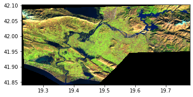
from ml4floods.visualization import plot_utils
plot_utils.plot_swirnirred_image(exported_files[0], size_read=600)
<AxesSubplot:>
Step 6: Run inference on the image time series#
Now, we’re going to iteratively load all the images that we’ve downloaded and run inference to compute flood extent estimations on them. See the Run inference notebook for a detailed tutorial on this.
First we need to download the model cofig and the model weights. If you’re running this tutorial in Google Colab you need to ‘add a shortcut to your Google Drive’ from the public Google Drive folder:
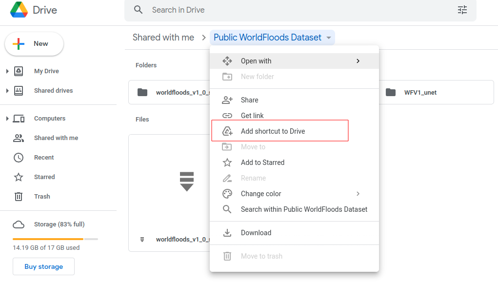
Then, mount that directory with the following code:
try:
from google.colab import drive
drive.mount('/content/drive')
assert os.path.exists('/content/drive/My Drive/Public WorldFloods Dataset'), "Add a shortcut to the publice Google Drive folder: https://drive.google.com/drive/u/0/folders/1dqFYWetX614r49kuVE3CbZwVO6qHvRVH"
google_colab = True
path_to_dataset_folder = '/content/drive/My Drive/Public WorldFloods Dataset'
dataset_folder = os.path.join(path_to_dataset_folder, "worldfloods_v1_0_sample")
experiment_name = "WFV1_unet"
folder_name_model_weights = os.path.join(path_to_dataset_folder, experiment_name)
except ImportError as e:
print(e)
print("Setting google colab to false, it will need to install the gdown package!")
google_colab = False
No module named 'google.colab'
Setting google colab to false, it will need to install the gdown package!
Alternatively,you can do this programatically using the the gdown package. For other alternatives see download WorldFloods.
import os
if not google_colab:
experiment_name = "WFV1_unet"
path_to_dataset_folder = 'worldfloods_v1_0_sample'
folder_name_model_weights = os.path.join(path_to_dataset_folder, experiment_name)
if not os.path.exists(folder_name_model_weights):
import gdown
gdown.download_folder(id="1Oup-qVD1U-re3lIQkw7TOKJsdu90blsk", quiet=False, use_cookies=False,
output=folder_name_model_weights)
# gdown.download(id="1mDQUzVL45_GTiILSDNeb-UN8xNROsKyC", output="WFV1_unet/model.pt", quiet=False)
Second we will load the model and the inference_function that tiles the Sentinel-2 image to run inference over those tiles.
from ml4floods.models.config_setup import get_default_config
from ml4floods.models.model_setup import get_model
from ml4floods.models.model_setup import get_model_inference_function
# Downlink the model weights and config from GDrive!
config_fp = os.path.join(folder_name_model_weights,"config.json")
config = get_default_config(config_fp)
# The max_tile_size param controls the max size of patches that are fed to the NN. If you're in a memory constrained environment set this value to 128
config["model_params"]["max_tile_size"] = 128
config["model_params"]['model_folder'] = path_to_dataset_folder
config["model_params"]['test'] = True
model = get_model(config.model_params, experiment_name)
model.to("cuda")
inference_function = get_model_inference_function(model, config,apply_normalization=True)
Loaded Config for experiment: WFV1_unet
{ 'data_params': { 'batch_size': 32,
'bucket_id': 'ml4floods',
'channel_configuration': 'all',
'filter_windows': False,
'input_folder': 'S2',
'loader_type': 'local',
'num_workers': 8,
'path_to_splits': '/worldfloods/public',
'target_folder': 'gt',
'test_transformation': { 'normalize': True,
'num_classes': 3,
'totensor': True},
'train_test_split_file': 'worldfloods/public/train_test_split.json',
'train_transformation': { 'normalize': True,
'num_classes': 3,
'totensor': True},
'window_size': [256, 256]},
'deploy': False,
'experiment_name': 'WFV1_unet',
'gpus': '0',
'model_params': { 'hyperparameters': { 'channel_configuration': 'all',
'label_names': [ 'land',
'water',
'cloud'],
'lr': 0.0001,
'lr_decay': 0.5,
'lr_patience': 2,
'max_epochs': 25,
'max_tile_size': 256,
'model_type': 'unet',
'num_channels': 13,
'num_classes': 3,
'val_every': 1,
'weight_per_class': [ 1.93445299,
36.60054169,
2.19400729]},
'model_folder': 'gs://ml4cc_data_lake/0_DEV/2_Mart/2_MLModelMart',
'path_to_weights': 'checkpoints/',
'test': False,
'train': True,
'use_pretrained_weights': False},
'resume_from_checkpoint': False,
'seed': 12,
'test': False,
'train': False,
'wandb_entity': 'ml4floods',
'wandb_project': 'worldfloods'}
Loaded model weights: worldfloods_v1_0_sample/WFV1_unet/model.pt
Getting model inference function
import torch
from ml4floods.data.worldfloods import dataset
from ml4floods.models.model_setup import get_channel_configuration_bands
import matplotlib.pyplot as plt
from ml4floods.visualization import plot_utils
from tqdm import tqdm
import numpy as np
from ml4floods.models import postprocess
import geopandas as gpd
channels = get_channel_configuration_bands(config.model_params.hyperparameters.channel_configuration)
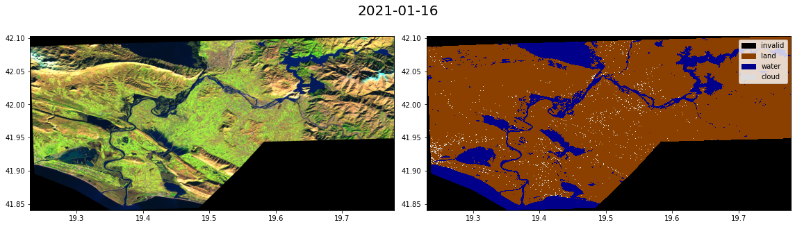
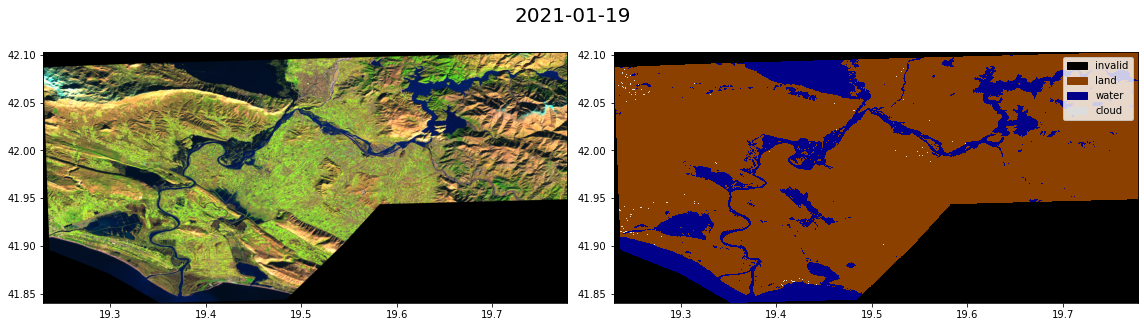
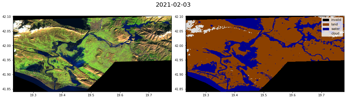
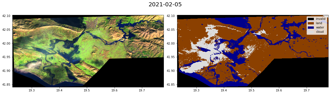
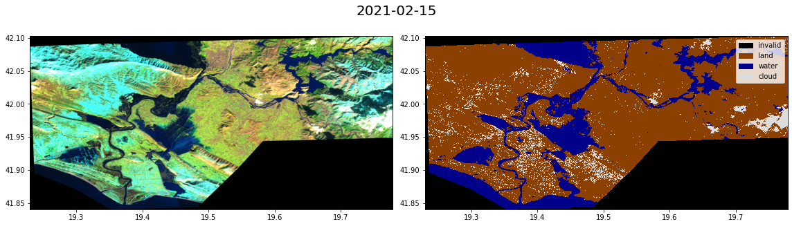
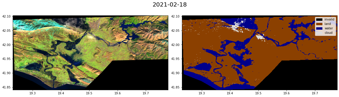
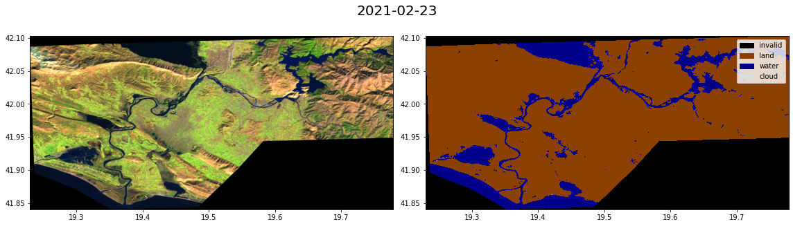
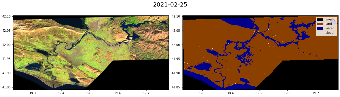
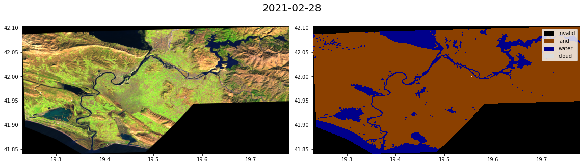
Here we loop over the images, making preditions and plotting both the Sentinel-2 image and the prediction.
%%time
folder_save = "ts_outputs"
os.makedirs(folder_save, exist_ok=True)
for filename in tqdm(exported_files):
# Load input in memory
torch_inputs, transform = dataset.load_input(filename, window=None, channels=channels)
# Make predictions
outputs = inference_function(torch_inputs.unsqueeze(0))[0] # (num_classes, h, w)
prob_water_mask = outputs[1].cpu().numpy()
binary_water_mask = prob_water_mask>.5
prediction = torch.argmax(outputs, dim=0).long() # (h, w)
mask_invalid = torch.all(torch_inputs == 0, dim=0)
prediction+=1
prediction[mask_invalid] = 0
name_plot = os.path.splitext(os.path.basename(filename))[0]
# Vectorize the output
geoms_polygons = postprocess.get_water_polygons(binary_water_mask, transform=transform)
vectorized_dataframe = gpd.GeoDataFrame({"geometry": geoms_polygons, "id": np.arange(len(geoms_polygons))})
vectorized_dataframe.to_file(f"{folder_save}/{name_plot}.geojson", driver='GeoJSON')
# Plot results
fig, axs = plt.subplots(1,2, figsize=((16,4.5)))
plot_utils.plot_swirnirred_image(torch_inputs, transform=transform, ax=axs[0])
plot_utils.plot_gt_v1(prediction.unsqueeze(0),transform=transform, ax=axs[1])
fig.suptitle(datetime.strptime(filename[-12:-4],"%Y%m%d").strftime("%Y-%m-%d"),fontsize=20)
plt.tight_layout()
fig.savefig(f"{folder_save}/{name_plot}.jpg")
fig.show()
0%| | 0/9 [00:00<?, ?it/s]/home/gonzalo/miniconda3/envs/ml4floods/lib/python3.9/site-packages/geopandas/io/file.py:362: FutureWarning: pandas.Int64Index is deprecated and will be removed from pandas in a future version. Use pandas.Index with the appropriate dtype instead.
pd.Int64Index,
<timed exec>:31: UserWarning: Matplotlib is currently using module://matplotlib_inline.backend_inline, which is a non-GUI backend, so cannot show the figure.
11%|██████████████████▋ | 1/9 [02:00<16:07, 120.99s/it]/home/gonzalo/miniconda3/envs/ml4floods/lib/python3.9/site-packages/geopandas/io/file.py:362: FutureWarning: pandas.Int64Index is deprecated and will be removed from pandas in a future version. Use pandas.Index with the appropriate dtype instead.
pd.Int64Index,
<timed exec>:31: UserWarning: Matplotlib is currently using module://matplotlib_inline.backend_inline, which is a non-GUI backend, so cannot show the figure.
22%|█████████████████████████████████████▎ | 2/9 [04:03<14:12, 121.82s/it]/home/gonzalo/miniconda3/envs/ml4floods/lib/python3.9/site-packages/geopandas/io/file.py:362: FutureWarning: pandas.Int64Index is deprecated and will be removed from pandas in a future version. Use pandas.Index with the appropriate dtype instead.
pd.Int64Index,
<timed exec>:31: UserWarning: Matplotlib is currently using module://matplotlib_inline.backend_inline, which is a non-GUI backend, so cannot show the figure.
33%|████████████████████████████████████████████████████████ | 3/9 [05:51<11:34, 115.69s/it]/home/gonzalo/miniconda3/envs/ml4floods/lib/python3.9/site-packages/geopandas/io/file.py:362: FutureWarning: pandas.Int64Index is deprecated and will be removed from pandas in a future version. Use pandas.Index with the appropriate dtype instead.
pd.Int64Index,
<timed exec>:31: UserWarning: Matplotlib is currently using module://matplotlib_inline.backend_inline, which is a non-GUI backend, so cannot show the figure.
44%|██████████████████████████████████████████████████████████████████████████▋ | 4/9 [07:48<09:39, 115.97s/it]/home/gonzalo/miniconda3/envs/ml4floods/lib/python3.9/site-packages/geopandas/io/file.py:362: FutureWarning: pandas.Int64Index is deprecated and will be removed from pandas in a future version. Use pandas.Index with the appropriate dtype instead.
pd.Int64Index,
<timed exec>:31: UserWarning: Matplotlib is currently using module://matplotlib_inline.backend_inline, which is a non-GUI backend, so cannot show the figure.
56%|█████████████████████████████████████████████████████████████████████████████████████████████▎ | 5/9 [09:41<07:40, 115.04s/it]/home/gonzalo/miniconda3/envs/ml4floods/lib/python3.9/site-packages/geopandas/io/file.py:362: FutureWarning: pandas.Int64Index is deprecated and will be removed from pandas in a future version. Use pandas.Index with the appropriate dtype instead.
pd.Int64Index,
<timed exec>:31: UserWarning: Matplotlib is currently using module://matplotlib_inline.backend_inline, which is a non-GUI backend, so cannot show the figure.
67%|████████████████████████████████████████████████████████████████████████████████████████████████████████████████ | 6/9 [11:39<05:47, 115.98s/it]/home/gonzalo/miniconda3/envs/ml4floods/lib/python3.9/site-packages/geopandas/io/file.py:362: FutureWarning: pandas.Int64Index is deprecated and will be removed from pandas in a future version. Use pandas.Index with the appropriate dtype instead.
pd.Int64Index,
<timed exec>:31: UserWarning: Matplotlib is currently using module://matplotlib_inline.backend_inline, which is a non-GUI backend, so cannot show the figure.
78%|██████████████████████████████████████████████████████████████████████████████████████████████████████████████████████████████████▋ | 7/9 [13:40<03:55, 117.57s/it]/home/gonzalo/miniconda3/envs/ml4floods/lib/python3.9/site-packages/geopandas/io/file.py:362: FutureWarning: pandas.Int64Index is deprecated and will be removed from pandas in a future version. Use pandas.Index with the appropriate dtype instead.
pd.Int64Index,
<timed exec>:31: UserWarning: Matplotlib is currently using module://matplotlib_inline.backend_inline, which is a non-GUI backend, so cannot show the figure.
89%|█████████████████████████████████████████████████████████████████████████████████████████████████████████████████████████████████████████████████████▎ | 8/9 [15:40<01:58, 118.54s/it]/home/gonzalo/miniconda3/envs/ml4floods/lib/python3.9/site-packages/geopandas/io/file.py:362: FutureWarning: pandas.Int64Index is deprecated and will be removed from pandas in a future version. Use pandas.Index with the appropriate dtype instead.
pd.Int64Index,
<timed exec>:31: UserWarning: Matplotlib is currently using module://matplotlib_inline.backend_inline, which is a non-GUI backend, so cannot show the figure.
100%|████████████████████████████████████████████████████████████████████████████████████████████████████████████████████████████████████████████████████████████████████████| 9/9 [17:40<00:00, 117.79s/it]
CPU times: user 16min 4s, sys: 4min 34s, total: 20min 38s
Wall time: 17min 40s
Step 7: Show vectorized floodmaps and S2 images in an interactive map#
In the final step we show the vectorized floodmaps over an interactive map using the geemap package.
Map = geemap.Map()
imgs_list = img_col.toList(n_images_col, 0)
for i in range(n_images_col):
if img_col_info_local.iloc[i]["cloud_probability"] > 75:
continue
img_show = ee.Image(imgs_list.get(i))
date_iter = img_col_info_local['system:time_start'][i]
Map.addLayer(img_show.clip(pol),
{"min":0, "max":3000,
"bands":["B11","B8","B4"]},
f"{date_iter.strftime('%Y-%m-%d')} S2 SWIR/NIR/RED",
True)
name_plot = f"albania_ts_{date_iter.strftime('%Y%m%d')}"
floodmap = gpd.read_file(f"{folder_save}/{name_plot}.geojson")
name = f"FloodMap {date_iter.strftime('%Y-%m-%d')}"
floodmap_folium = folium.features.GeoJson(floodmap, name=name, show=False)
Map.add_child(floodmap_folium, name=name)
# Show JRC permanent water layer
visualization = {
"bands": ['waterClass'],
"min": 0.0,
"max": 3.0,
"palette": ['cccccc', 'ffffff', '99d9ea', '0000ff']
}
Map.addLayer(permanent_water_img, visualization, name="JRC Permanent water")
Map.addLayer(pol, {"color": 'FF000000'}, "AoI")
Map.centerObject(pol, zoom=11)
folium.LayerControl(collapsed=False).add_to(Map)
Map